Operating a Fuel Cell Stack
Introduction
You might have just purchased your first fuel cell and are now asking yourself: How should I operate it? How do I measure its performance? What are the limiting factors reducing the stack performance? If this is the case, this blog is for you. The aim of this blog is to familiarize yourself with fuel cell performance measurements, identifying performance issues, and the application of appropriate operating conditions.
Measuring the performance of a fuel cell and identifying performance losses
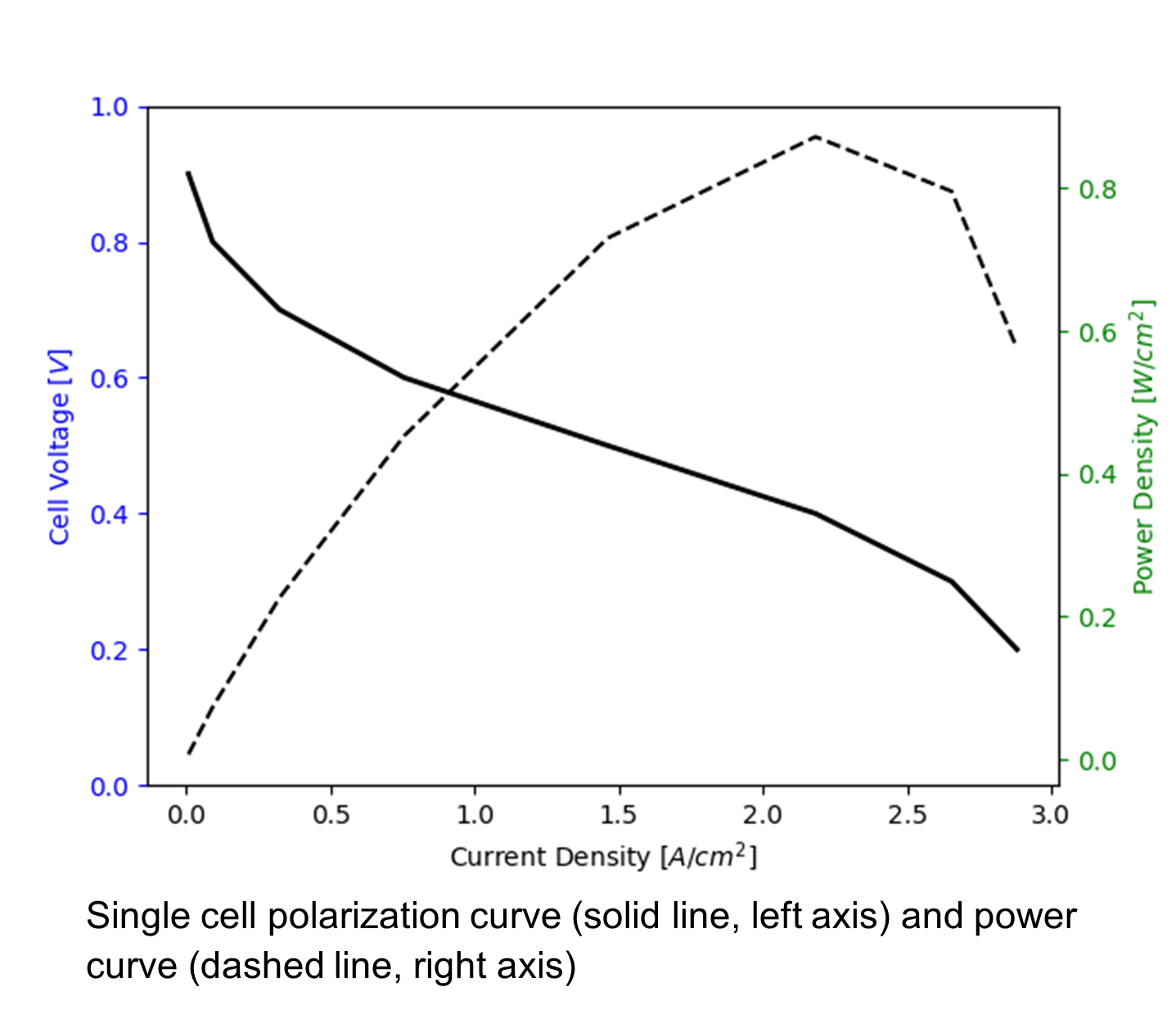
The performance of a fuel cell stack is usually measured by its polarization curve, i.e., a curve relating stack voltage, in V, to current, in A. By multiplying the cell voltage by the current, a stack power curve can also be obtained relating the stack power, in W, to the stack current. For single cells, the polarization and power curves are usually measured as cell voltage vs. current density, in A/cm2, and power density, in W/cm2, where the area is the geometrical area of the cell. A typical single cell polarization and power curves are shown below.
In order to obtain a polarization curve, a hydrogen fuel cell, heated at a specified temperature, is supplied with hydrogen and air at a given flow rate, relative humidity and pressure, and either the current density is recorded at varying cell voltage (potentiostatic) or the voltage is recorded at varying current density (galvanostatic). The current vs voltage measurement is usually performed either with a potentiostat, such as Biologic SP-300 or Scribner 885, or an electrical load, such as Scribner 890, usually integrated in the test station. Cell temperature and gas flow rates and humidities are controlled with a fuel cell test station, such as Scribner 850 or Greenlight Innovation G20 .
An ideal fuel cell would be able to maintain the theoretical cell voltage at any current (note that, for a fuel cell operating with hydrogen and air at 80 ℃, the theoretical cell voltage is 1.18 V). In this case, the fuel cell would be operating at its theoretical efficiency of 1.18/1.48 = 0.8. Unfortunately, as it can be observed on the typical polarization curve above, the cell voltage is reduced as current increases. The voltage losses are due to kinetic, ohmic and mass transport losses.
Kinetic losses dominate at low current density and are responsible for the initial drop in performance. These are mainly due to the sluggish oxygen reduction reaction in the cathode. The voltage drop due to the reaction, considering the losses are reasonably large, can be estimated using a modified Tafel equation in order to account for cross-over, i.e.,
\[E_{kin} = {RT \over \alpha F}ln \left(\frac{i + i_n}{i_o} \right) \]where R is the universal ideal gas constant, T is the cell temperature, F is Faraday’s constant, α is the Tafel coefficient, in is the hydrogen cross-over current and io is the exchange current density which depends on temperature, i.e.,
\[i_o = i_o(T_o)exp \left(-E_a \left(\frac{1}{T} - \frac{1}{T_0} \right)\right) \]where Ea is the activation energy of the reaction. Even though the most influential parameter controlling this loss is the catalyst (the Tafel coefficient and exchange current density depend on the catalyst), operating conditions can be adjusted to reduce this loss since the exchange current density increases with increasing temperature.
At moderate current densities, voltage losses due to the transport of protons across the membrane and electrons from the current collectors to the reaction site start to also become important. These losses are characterized by Ohm’s law such that the value of the Ohmic losses, Eohmic, is
\[E_{ohmic} \approx (R^{H^+}_{PEM} + R^{e^-}_{GDL} + R^{e^-}_{BP} + R^{e^-}_{CC})i = R_{cell}i\]where the first term in the parenthesis represents the membrane resistance, which depends nonlinearly on membrane humidity and cell temperature, and the other three terms represent gas diffusion layer, bipolar plate and current collector electronic resistances, which are constant. Despite the nonlinear membrane resistance, these losses are usually identified by the linear region in the polarization curve between voltage and current density. In this linear region, the cell resistance can be approximated by measuring the slope of the polarization curve. Two more accurate experimental techniques to measure the cell resistance are current interrupt and impedance spectroscopy [1]. Using impedance spectroscopy, kinetic and ohmic losses can both be estimated with the aid of an equivalent-circuit or a physics based model. Considering that the conductivity of the proton conductive membrane depends strongly on the humidity of the cell [2], operating conditions will strongly influence ohmic losses.
Finally, the sharp drop in performance observed at high current density, i.e., at above 2.5 A/cm2 in the example above, is usually due to mass transport limitations. These can appear in both anode and cathode but are most common in the cathode. They might occur for three reasons: 1) inadequate flow rate to the cell at either anode or cathode, 2) macroscopic transport losses due to water accumulation in the electrode, usually the cathode; and, 3) microscopic transport losses due to local oxygen transport resistances as the oxygen molecule moves from the gas pores to the reaction sites through ionomer and water films usually covering the reaction sites on the catalyst surface. In order to identify if these losses are responsible for the reduced performance a well known experimental method is to replace air by helox, i.e., a mixture of helium and oxygen (21 %vol.). An analytical expression to predict these losses is difficult to obtain as it depends on many physical processes, as an approximation, the following expression can be used, i.e.,
\[E_{mass} \approx Aln \left( 1 - \frac{i}{i_L} \right)\]where A and iL are coefficients that can be obtained experimentally. Again, operating conditions are critical to mitigating these effects by providing appropriate flow rate and controlling the degree of humidification in the cell to prevent water build-up, for example, as observed in ref [3].
In summary, the polarization curve dictates the performance of a fuel cell. It can be approximated with the following expression, i.e.,
\[E_{cell} \approx E^o - \frac{RT}{\alpha F} exp \left( \frac{i + i_n}{i_0} \right) - R_{cell} i - A ln \left( 1 - \frac{i}{i_L} \right)\]Where Rcell is the sum of all ohmic resistances (see above). As current increases, the voltage decreases due to kinetic, ohmic and transport losses. The reduced voltage leads to a reduction in efficiency, which can be computed as the cell voltage divided by 1.48 V, and to a reduction in maximum peak power. These losses result in the generation of heat inside the cell, which is given by
\[\dot{Q} = (E_{cell} - 1.48)i \]Cell voltage losses can be mitigated with proper selection of operating conditions for a given cell as discussed below.
Selection of appropriate operating conditions
The most critical operating conditions in a fuel cell stack are the cell temperature, and the fuel and reactant gas flow rate, relative humidity and pressure. Not all these parameters can always be controlled in a stack as we will discuss later. Let’s first assume that all of them can be controlled.
Fuel Flow Rate
Fuel and reactant flow rate are the most important parameters to control as hydrogen starvation could result in irreparable damage to the stack due to carbon corrosion [4]. It is recommended that before connecting the stack to a load, hydrogen is circulated through the stack for a few minutes to make sure the hydrogen channel is completely filled with hydrogen. In order to determine the appropriate flow rate, Faraday’s law can be used. It states that the consumed molar flux of fuel/reactant, Ni, must be equal to the current, I, over the number of moles of electrons per mole of fuel/reactant, ni, times Faraday’s constant, F (96,485 C/mol e), i.e.,
\[N_{i}= {I \over n_iF}\]In this case, using the molar mass, Mi, to convert from molar to mass flow rate, the minimum mass flow rate of dry hydrogen and air is (I*MH2)/(2*F) while that of dry air is (0.21*I*MO2)/(4*F) in g/s (assuming Mi is written in g/mol). Using this flow rate, there would not be any hydrogen and oxygen left at the stack exit; therefore, the flow rate is usually selected to be a multiple of this number, known as the stoichiometry. The hydrogen stochiometry is usually between 1 and 2, while the air stoichiometry is usually higher in order to mitigate oxygen mass transport losses due to the smaller concentration gradient and water accumulation.
Temperature and Humidity
Cell temperature influences reaction kinetics, membrane conductivity and heat rejection from the stack. Elevated temperatures improves the reaction kinetics; however, it makes it more difficult to maintain the proton conductivity membrane hydrated. Furthermore, at about 120-140 C Nafion membranes undergo a change in morphology that changes its properties, including a reduction in proton conductivity. Considering the above, fuel cells using humidified gases are commonly operated at approximately 80 C, as this provides adequate kinetics and membrane hydration can still be maintained due to gas humidification. Fuel cell stacks that do not humidify the hydrogen and air streams are more likely to operate at lower temperatures as it is easier to humidify the gases, but at the expense of increased kinetic losses.
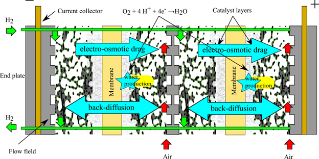
Reaction/fuel relative temperature and humidity both influence cell hydration; therefore, their optimization requires understanding the water balance in the cell, known as water management. In order to effectively conduct protons, the electrolyte (usually Nafion) must be well hydrated; however, liquid water accumulation in the cell results in reactant mass transport losses. At low current densities, cell hydration is mainly controlled by the relative humidity of the cell, therefore ohmic losses are minimized by supplying the fuel cell with fully humidified gases. Unfortunately, as the cell current density increases water is produced in the cathode and dragged from anode to cathode via electro-osmotic drag, a process where protons transport with them one to two water molecules. These two mechanisms lead to water accumulation in the cathode, despite water diffusion through the membrane trying to move water back towards the anode when the concentration in the cathode is higher(see figure below). If water is allowed to accumulate in the cathode, it will block the transport pathways for oxygen to reach the reaction site, leading to the mass transport losses discussed above. In order to establish a balance between proper hydration at low currents and limited flooding at high currents, an optimal relative humidity needs to be identified for the given cell. In our laboratory, a relative humidity of approximately 70% appears to give good results when the cell temperature is 80 C and the pressure in anode and cathode is 1.5 atmospheres (absolute) [3]. Optimization of the cell temperature and relative humidity to achieve a good water balance is critical.
Pressure
The last parameter that requires optimization is the pressure. High fuel and reactant pressures result in a higher cell voltage and reduced transport losses, therefore it is usually beneficial to operate the fuel cell under pressure; however, operation at high pressure increases hydrogen crossover, and increasing air pressure requires the use of a compressor. Furthermore, operating anode and cathode at different pressures might result in membrane damage. Therefore, the operating pressure requires establishing a tradeoff between the investment on a compressor and the energy to run it, and the increased performance.
Controlling hydrogen and air flow rates, humidity and pressure, as well as cell temperature require the use of external devices such as mass flow controllers and humidifiers. In many applications, operating the fuel cell at sub-optimal conditions and eliminating the use of external devices might be preferable. For example, small stacks might run with a dead-ended anode, where the cell hydrogen outlet is closed with an exhaust valve and hydrogen enters the cell only due to a pressure gradient that is established as the fuel is consumed. In this case, neither the anode flow rate nor its humidity are controlled, and the only parameter used to control the anode flow is when to open/close the exhaust valve, known as the purge cycle. Optimization of the purge cycle is important as nitrogen and water will accumulate at the end of the channel over time and the exhaust valve must be opened to expose the end of the channel to fresh hydrogen. Similarly, the cathode flow rate is carefully controlled in automotive and heavy-duty transportation stacks, however in smaller applications, an open cathode, also known as air breathing, configuration is sometimes used where a fan is used to draw unconditioned atmospheric air into the cathode channels.
Conclusions
In summary, the performance of a fuel cell can be characterized by its polarization curve, a curve relating cell voltage to current. The aim of a fuel cell engineer is to achieve the highest voltage at the desired current density in order to increase fuel cell efficiency and reduce cooling requirements. To achieve this goal, hydrogen and air flow rates, humidity and pressure, as well as cell temperature should be carefully controlled and optimized.
Marc Secanell
Professor of Mechanical Engineering

Marc Secanell is a Professor in the Department of Mechanical Engineering at the University of Alberta, Canada, and the director of the Energy Systems Design Laboratory. He received his Ph.D. and M.Sc. in Mechanical Engineering from the University of Victoria, Canada, in 2008 and 2004, respectively. He holds a B.Eng. degree (2002) from the Universitat Politècnica de Catalunya (BarcelonaTech). In 2008, he was an Assistant Research Officer at the National Research Council of Canada, Institute for Fuel Cell Innovation in Vancouver, Canada, and 2015-16 and 2022-23 he was a visiting research scholar in the Energy Conversion Division at the Lawrence Berkeley National Laboratory (US) and at Johnson Matthey Technology Center (UK) respectively. He has authored over 80 journal articles, 30 conference proceedings and four book chapters receiving over 4,000 citations (h-index: 38 in Google Scholar).
Google Scholar: https://scholar.google.ca/citations?user=NjRIwW0AAAAJ&hl=en
References
[1] Cooper and Smith, Journal of Power Sources 160 (2006) 1088–1095 https://doi.org.
[2] Peron et al., Journal of Membrane Science 356 (2010) 44–51 (https://doi.org).
[3] Wei et al., Chemical Engineering Journal 471 (2023) 144423 https://doi.org).
[4] Zhao et al, Journal of Power Sources, 488 (2021) 229434 (https://doi.org)